XG Boost #

• Extreme Gradient Boosting
• 대용량 분산 처리를 위한 Gradient Boosting 라이브러리
• Decision Tree(의사결정나무) 에 Boosting 기법을 적용한 알고리즘
• AdaBoost는 학습 성능은 좋으나, 모델의 학습 시간이 오래 걸리는 단점
• 병렬 처리 기법을 적용하여 Gradient Boost보다 학습 속도를 끌어올림
• Hyper-Parameter가 너무 많기 때문에 권장 세팅 사용 @ http://j.mp/2PukeTS

Decision Tree #

• 이해하기 쉽고 해석도 용이함
• 입력 데이터의 작은 변동에도 Tree의 구성이 크게 달라짐
• 과적합이 쉽게 발생 (중간에 멈추지 않으면 Leaf 노드에 하나의 데이터만 남게 됨)
• 의사결정나무의 문제를 해결하기 위해 Boosting 기법 활용
• ex) 테니스를 쳤던 과거 데이터를 보고 날씨 정보를 이용해 의사결정

AdaBoost #

• Adaptive Boosting
• 데이터를 바탕으로 여러 weak learner 들을 반복적으로 생성
• 앞선 learner가 잘못 예측한 데이터에 가중치를 부여하고 학습
• 최종적으로 만들어진 strong learner를 이용하여 실제 예측 진행
• 에러를 최소화하는 weight를 매기기 위해 경사 하강법 사용
• ex) Regression: 평균/가중평균, Classification: 투표

XG Boost References #

• NGBoost Explained (Comparison to LightGBM and XGBoost)
• Gradient Boosting Interactive Playground
• Gradient Boosting explained
• Comparison for hyperparams of XGBoost & LightGBM
• XGBoost Parameters
• XG Boost 하이퍼 파라미터 상세 설명
• Complete Guide to Parameter Tuning in XGBoost (with python codes)
• Microsoft EBM (Explainable Boosting Machine)
• 정형데이터를 위한 인공신경망 모델, TabNet

Ensemble #

• 주어진 데이터를 이용하여 여러 개의 서로 다른 예측 모형을 생성한 후,
  예측 모형의 예측 결과를 종합하여 하나의 최종 예측결과를 도출해내는 방법
• 다양한 모델이 문제 공간의 다른 측면을 보면서 각기 다른 방식으로 오점이 있다고 가정
  (모델 별로 약점을 보완)

Boosting #

• weak learner들을 strong learner로 변환시키는 알고리즘
  (약한 학습기를 여러개 사용해서 하나의 강건한 학습기를 만들어내는 것)
• 의사결정나무 모델을 합리적인 수준(60~70% 성능)에서 여러 종류 생성
• ex) AdaBoost

Gradient Boosting #

• 경사 하강법을 사용해서 AdaBoost보다 성능을 개선한 Boosting 기법
• AdaBoost는 높은 가중치를 가진 지점이 존재하게 되면 성능이 크게 떨어지는 단점
  (높은 가중치를 가진 지점과 가까운 다른 데이터들이 잘못 분류될 가능성이 높음)
• Gradient Boosting 기법은 이전 모델에 종속적이기 때문에 병렬 처리가 불가능

Bagging #

• Bootstrap Aggregating
• 가중치를 매기지 않고 각각의 모델이 서로 독립적
• x 데이터 열들의 서로 다른 조합으로 독립적인 모델을 여러 종류 생성
• ex) Random Forest

Random Forest #

• 각 모델은 서로 다른 샘플 데이터셋을 활용 (Bootstrap Sampling & Bagging)
• 각 데이터셋은 복원추출을 통해 원래 데이터셋 만큼의 크기로 샘플링 (누락 & 중복 발생)
• 위 서로 다른 샘플로 각 모델 생성 시, 각 노드 지점마다 x열 n개 중 랜덤하게 m개 중 분기 선택
• Classification에서는 root n을 m으로 사용
• Regression에서는 n/3을 m으로 사용
• @ https://j.mp/3rZ05bN & https://j.mp/3GJ7QqH

Learning Process #

• @ https://j.mp/3jRJH6n

Import Libraries #

import numpy as np
import matplotlib.pyplot as plt

from sklearn import ensemble
from sklearn import datasets
from sklearn.utils import shuffle
from sklearn.metrics import mean_squared_error

Load Data #

boston = datasets.load_boston()

X, y = shuffle(boston.data, boston.target, random_state=13)
X = X.astype(np.float32)
offset = int(X.shape[0] * 0.9)

X_train, y_train = X[:offset], y[:offset]
X_test, y_test = X[offset:], y[offset:]

• load 부분에서 다른 데이터도 사용 가능
• boston.data: x data
• boston.target: y data
• int(X.shape[0] * 0.9): 전체 행 중 90 퍼센트 의미
• boston.feature_names: 데이터셋에서 열 이름
• boston.DESCR: 데이터에 대한 상세 설명

Model Fitting #

params = {'n_estimators': 500, 'max_depth': 4, 'min_samples_split': 2,
          'learning_rate': 0.01, 'loss': 'ls'}
clf = ensemble.GradientBoostingRegressor(**params)

clf.fit(X_train, y_train)
mse = mean_squared_error(y_test, clf.predict(X_test))
print("MSE: %.4f" % mse)

• **params: 딕셔너리를 파라미터로 변환 @ https://j.mp/2IPuJzY
• clf: Classifier

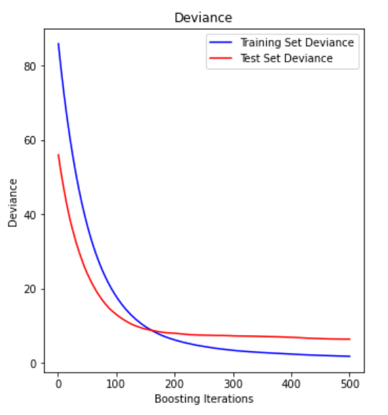
Plot Deviance #

test_score = np.zeros((params['n_estimators'],), dtype=np.float64)

for i, y_pred in enumerate(clf.staged_predict(X_test)):
    test_score[i] = clf.loss_(y_test, y_pred)

plt.figure(figsize=(12, 6))
plt.subplot(1, 2, 1)
plt.title('Deviance')
plt.plot(np.arange(params['n_estimators']) + 1, clf.train_score_, 'b-',
         label='Training Set Deviance')
plt.plot(np.arange(params['n_estimators']) + 1, test_score, 'r-',
         label='Test Set Deviance')
plt.legend(loc='upper right')
plt.xlabel('Boosting Iterations')
plt.ylabel('Deviance')

• Deviance: 편차값, 에러
• n_estimators: 의사결정나무 모델을 몇 개 만들었는지
• Test Data에 대한 에러 라인이 튕겨올라가는 지점이 Overfitting

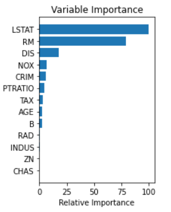
Plot Feature Importance #

feature_importance = clf.feature_importances_

feature_importance = 100.0 * (feature_importance / feature_importance.max())
sorted_idx = np.argsort(feature_importance)
pos = np.arange(sorted_idx.shape[0]) + .5
plt.subplot(1, 2, 2)
plt.barh(pos, feature_importance[sorted_idx], align='center')
plt.yticks(pos, boston.feature_names[sorted_idx])
plt.xlabel('Relative Importance')
plt.title('Variable Importance')
plt.show()

• feature_importances_: 트리 기반 모델이 가지고 있는 변수, 각각의 열마다의 중요도
• Feature Importance는 상대적인 중요도이기 때문에 합계가 1
• LSTAT(인구 중 하위 계층 비율)이 집값을 예측할 때 가장 중요함

Feature Importance References #

• Feature Importance Analysis (LIME)
• Permutation importance 한글 설명
• Permutation importance with Pipeline